Welcome to the
Info/Demo page for MATH 337,
Numerical Differential Equations!
When creating this page, I had in mind the following goals:
1. To describe the background
you will need to succeed in this course;
2. To describe what the course
will cover;
and
3. To demonstrate the level of
complexity of the problems that the students who had taken this course
were able to solve.
The first two goals are covered in the Info part of this page. To skip
that part and go directly to the Demos, which address the third goal,
click here.
Info
Background:
You will need to know the basic Calculus (especially
the Taylor series) and Linear Algebra (especially the eigenvalues). Any
knowledge of the ordinary differential equations (ODEs) beyond what is
commonly covered in Calculus, as well as familiarity with partial
differential equations (PDEs) and Fourier transform, will be
beneficial, but not critical
for succeeding in this course.
The other important ingredient is your willingness to program, although no
programming proficiency on your part is assumed. After all, the way to
solve most real-world problems is to program them into codes! The
programming language of the course is Matlab.
Course outline:
Part
I of the course will describe methods of solution of
initial-value problems for ODEs. This class of problems
arises when a scientists studies the development of some process in
time. Examples include evolution of the population of a biological
species, dynamics of a laser beam, motion of a charged particle in
electric and magnetic fields, etc.
Part I also lays down the mathematical background on which the other
material of this course will rest. Namely, the students learn how to
write numerical schemes whose solutions are guaranteed to closely approximate
the analytical solutions of the respective ODEs. This is quite
remarkable, considering that one usually does not know what that
analytical solution is!
Part II
will describe methods of solution of boundary values problems for ODEs.
Examples of this class of problems include finding the shape of a
loaded beam, a stationary temperature or heat flow distribution in a
reservoir, etc.
Finally, in Part III the students will
learn how to solve initial-value problems for partial differential
equations. This class of problems is similar to that studied in Part I,
with the modification being that now the process in question
develops differently in different regions of the space! The
applications include the heat transfer, traffic flow, propagation of
electric pulses in media with complex properties, etc.
The course does not specifically cover (due to the
lack of time) methods for modeling wave propagation. However, the
mathematical background that the course provides is amply sufficient
for the students to learn those methods on their own.
For the Final
Project, the students are offered a list of topics from
which they select the one they are most interested in. For
example, learning and applying one of the numerical methods to a wave
propagation problem may be one of such topics. As another example, the
second demo on this page was created by a student as his final project.
Students are also welcome to suggest their own problems they would like
to solve numerically.
For more
information, visit the main
page of this course.
The first
Demo illustrates that the knowledge of properties of a numerical
method is sometimes critical for the method's success, when it is
applied to a specific problem.
The movie below shows the evolution of a slightly damped
pendulum when computed by:
(a) a 2nd-order accurate modified Euler method and
(b) a 1st-order accurate symplectic Euler method.
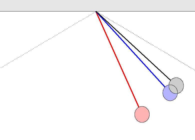
The color coding of the penduli is:
Exact solution:
Gray
Modified Euler
method: Pink
Symplectic Euler method:
Blue.
The dotted lines on the sides are the guides for the eye: They show the
maximum elevation of the top point of the pendulum without damping.
Click on the picture on the left to watch the movie of these penduli.
The movie size is 2.7 MB.
Usually, 2nd-order methods are more accurate than 1st-order ones. In
particular, the modified Euler method is widely used due to its
simplicity and relatively good accuracy. However, when applied to a
certain class of problems, this method can lead to totally wrong results.
Namely, note two things in the movie:
* The (supposedly more accurate) 2nd-order numerical solution
deviates farther from the exact solution than the 1st-order numerical
solution.
* The 2nd-order solution even gives qualitatively wrong information: It
shows that the amplitude of the pendulum slowly increases, whereas that
amplitude found from the exact solution slowly decreases!
Symplectic methods, to which the 1st-order method used above belongs,
are a hot topic both in mathematics and in applications. For example,
such methods are widely used in computer animation. Upon taking this
course, the students will learn the reason that causes symplectic
methods to outperform non-symplectic ones.
The movies shown in the second Demo
were created by Mr. Evan Flath, who took MATH 238 (a previous name for
MATH 337) in the Spring 2005.
Evan wrote a code that solves the following partial differential
equation in 2 spatial dimensions:

Even with modern computers, solution of PDEs in more than one spatial
dimensions may be quite time-consuming. Therefore, the course
emphasizes time-efficient
methods for such problems. Evan implemented one of such methods in his
code.
The above equation, known
as the complex Ginzburg-Landau equation, has been found to describe a
great variety of phenomena in physics, chemistry, and biology. Its
particular realization shown here describes the growth of a thin film
at the interface of two crystalline materials (see a paper by I.
Aranson et al, Phys.Rev.Lett. 80,
1770 (1998) for more details). The height of the film is modeled by the
argument of the complex-valued solution of the equation.
The movies depict
three (out of many more) scenarios of the film growth.
The first
movie shows the formation of a spiral out of a so-called screw
dislocation in the original film.
The second movie shows the
evolution of two spirals of the same orientation, whose centers have
drifted close to one another.
The third movie shows a
similar evolution in the case when the orientation of the spirals are
opposite.
To watch the movies, click on the corresponding pictures below. You may
need version 7 or later of QuickTime Player, which you can download for
free from the web.
Note
that the movies show contour plots of both the argument and the modulus
of the solution. As mentioned above, the argument models the film's
height, while the modulus has no independent physical meaning and is
shown only for completeness.
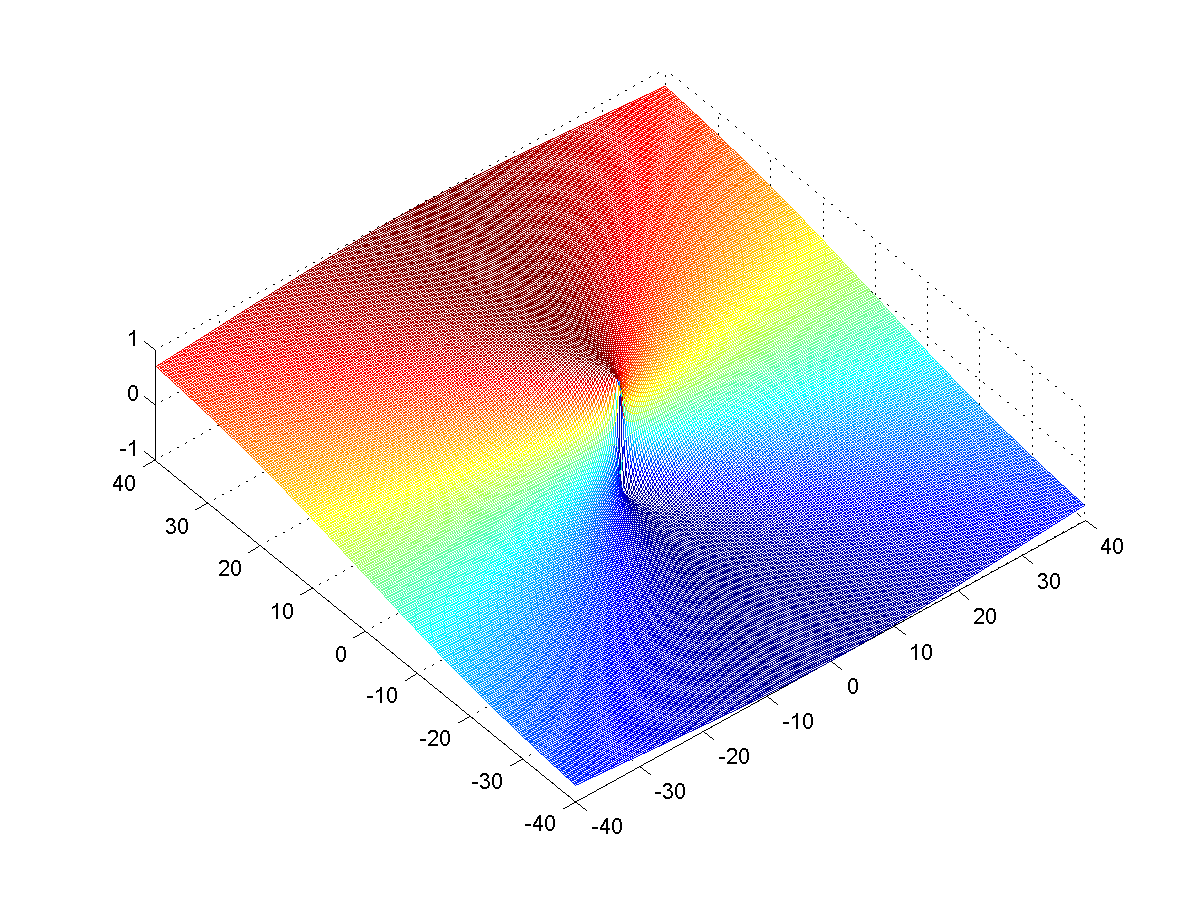
Initial condition:
Screw dislocation (no spirals).
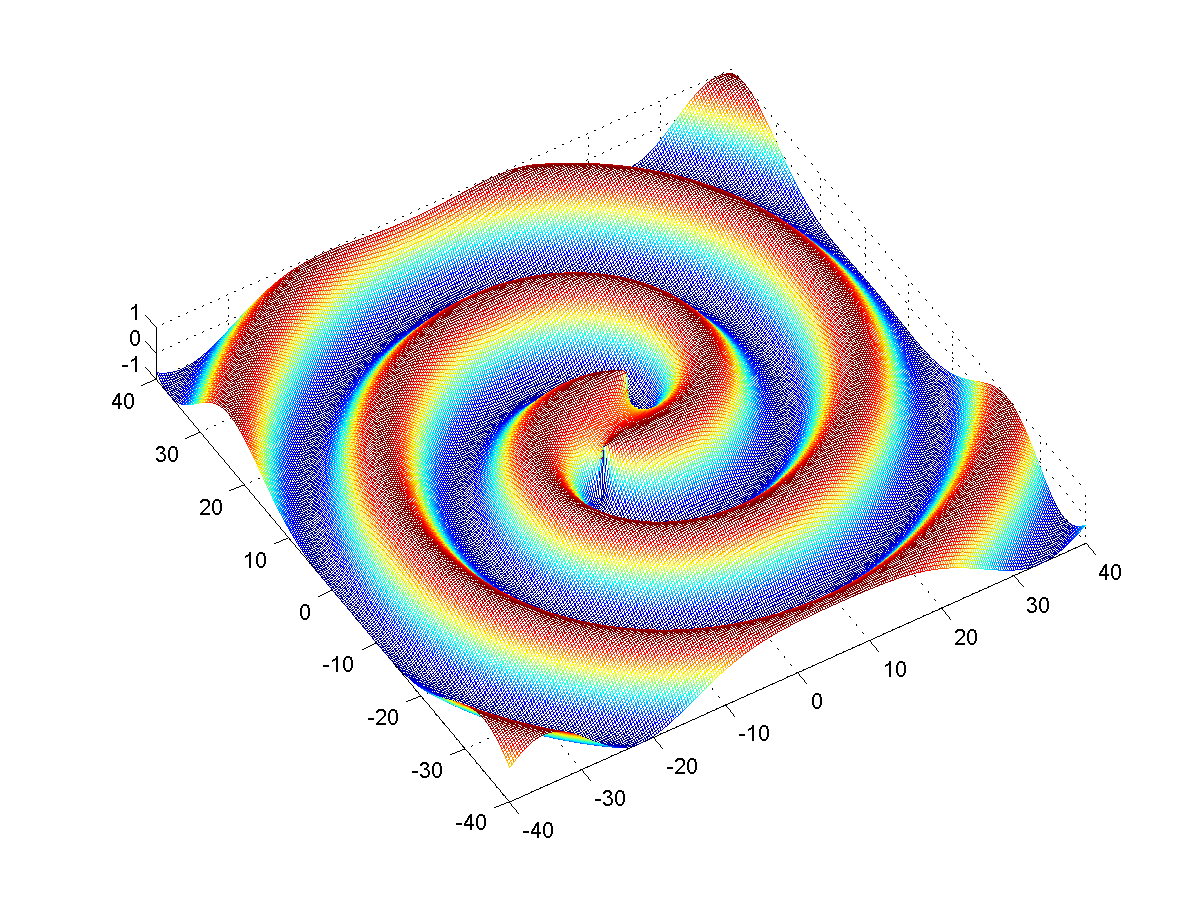
Initial condition:
Two spirals of equal orientation.
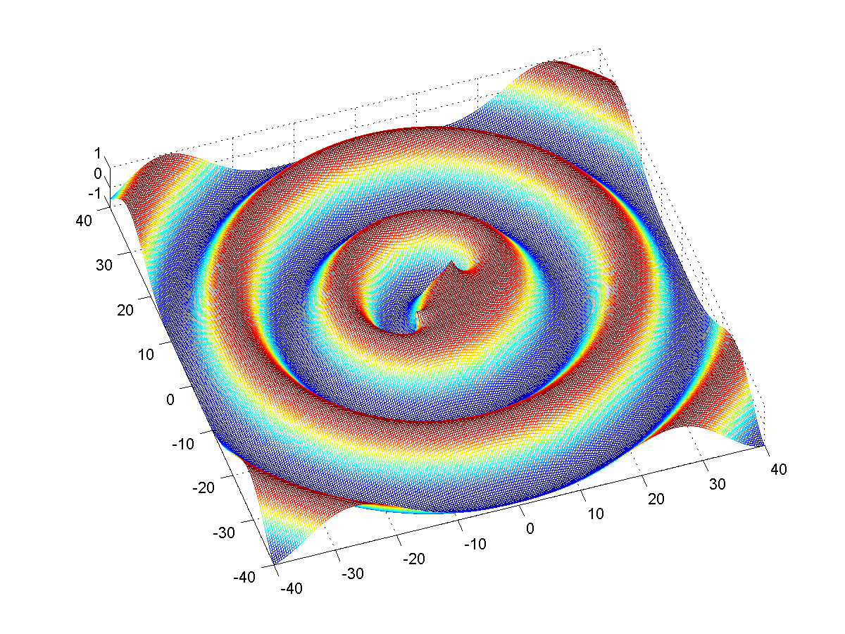
Initial condition:
Two spirals of
opposite orientation.
You might have noticed that the solution acquires with time a somewhat
square shape. This is the effect of the boundaries of the square
domain.
Back to the main page of MATH 337